
An introduction to GRF (getting started)

@misc{grf,
  title        = {grf},
  author       = {Athey and Tibshirani and Wager},
  howpublished = {\url{https://grf-labs.github.io/grf/}},
  note         = {Software / documentation}
}Follow the analysis.
Select a node to explore the method
Assemble X, W, Y; check overlap
Data preparation — shapes the raw inputs into what the estimator expects.
One row per unit; numeric design matrix X, treatment W, outcome Y. Eyeball propensity overlap.

Before using this step, make its assumptions and its output explicit. A useful peer note explains what you would check, what could go wrong, or what would change your interpretation.
Questions to explore- Which assumption matters most here, and what evidence could challenge it?
- What would you check before passing this output to the next step?
Choose a question to start your comment.
Peer discussion
- Bring your experience, a question, or a different perspective.
Log in to comment on this step.
[GRF] Regression forest
The core estimate — where the causal quantity itself is computed.
Fit E[Y|X]; read off OOB predictions and variable_importance().
Regression forest — Honest non-parametric regression for E[Y|X], with out-of-bag predictions and pointwise CIs.
rf <- regression_forest(X, Y)
Y.hat <- predict(rf)$predictions
Before using this step, make its assumptions and its output explicit. A useful peer note explains what you would check, what could go wrong, or what would change your interpretation.
Questions to explore- Which assumption matters most here, and what evidence could challenge it?
- What would you check before passing this output to the next step?
Choose a question to start your comment.
Peer discussion
- Bring your experience, a question, or a different perspective.
Log in to comment on this step.
[GRF] Quantile forest
The core estimate — where the causal quantity itself is computed.
Fit conditional quantiles to see distributional, not just mean, structure.
Quantile forest — Conditional quantile estimation — the full predictive distribution, not just the mean.
qf <- quantile_forest(X, Y, quantiles = c(.1, .5, .9))
predict(qf, X.test)
Before using this step, make its assumptions and its output explicit. A useful peer note explains what you would check, what could go wrong, or what would change your interpretation.
Questions to explore- Which assumption matters most here, and what evidence could challenge it?
- What would you check before passing this output to the next step?
Choose a question to start your comment.
Peer discussion
- Bring your experience, a question, or a different perspective.
Log in to comment on this step.
[GRF] Causal forest
The core estimate — where the causal quantity itself is computed.
Fit CATEs with the same call shape; predict with estimate.variance = TRUE.
Causal forest — Honest random forest for heterogeneous treatment effects — CATE for a binary treatment via GRF moment conditions.
cf <- causal_forest(X, Y, W)          # Y.hat, W.hat cross-fit
tau.hat <- predict(cf)$predictions    # OOB CATEs
Before using this step, make its assumptions and its output explicit. A useful peer note explains what you would check, what could go wrong, or what would change your interpretation.
Questions to explore- Which assumption matters most here, and what evidence could challenge it?
- What would you check before passing this output to the next step?
Choose a question to start your comment.
Peer discussion
- Bring your experience, a question, or a different perspective.
Log in to comment on this step.
OOB predictions & variable importance
Reporting — turn the numbers into a figure or table a reader can act on.
Compare the three forests; show importance and a CATE histogram.
Before using this step, make its assumptions and its output explicit. A useful peer note explains what you would check, what could go wrong, or what would change your interpretation.
Questions to explore- Which assumption matters most here, and what evidence could challenge it?
- What would you check before passing this output to the next step?
Choose a question to start your comment.
Peer discussion
- Bring your experience, a question, or a different perspective.
Log in to comment on this step.
Inputs & data
2,000 obs, 10 covariates X, a binary treatment W, continuous outcome Y.
Show data format & exampleHide example
Format — one row per unit. A covariate matrix X (numeric), a binary treatment W ∈ {0,1}, and an outcome Y.
  X1     X2    X3    W    Y
 0.42  -1.1   0     1   3.10
-0.07   0.6   1     0   1.85
 1.20   0.3   0     1   4.02
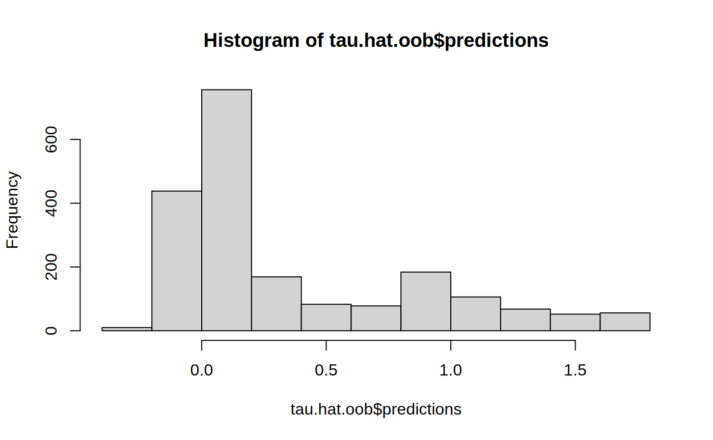
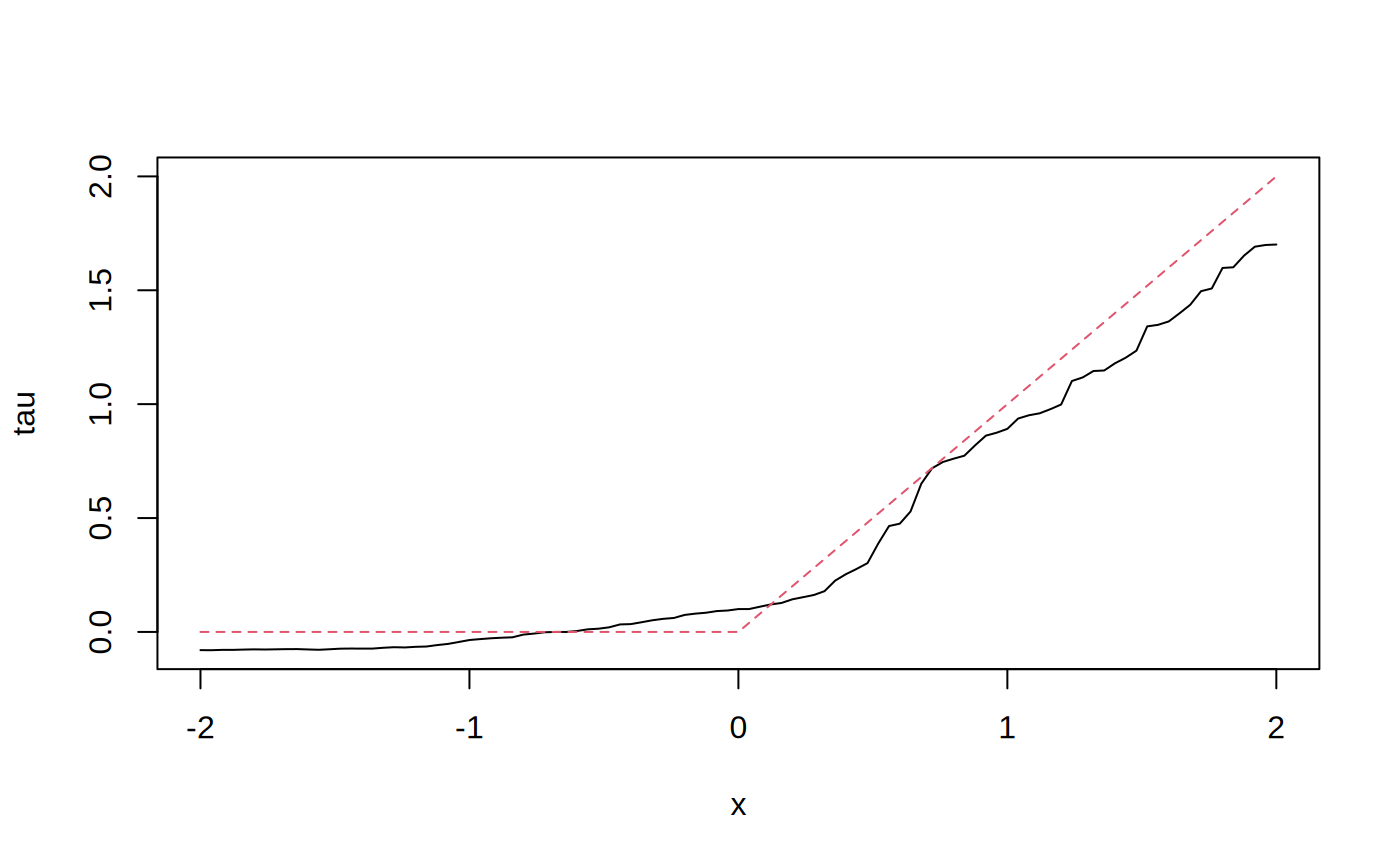
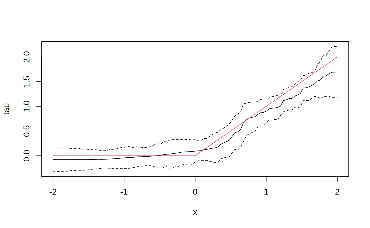
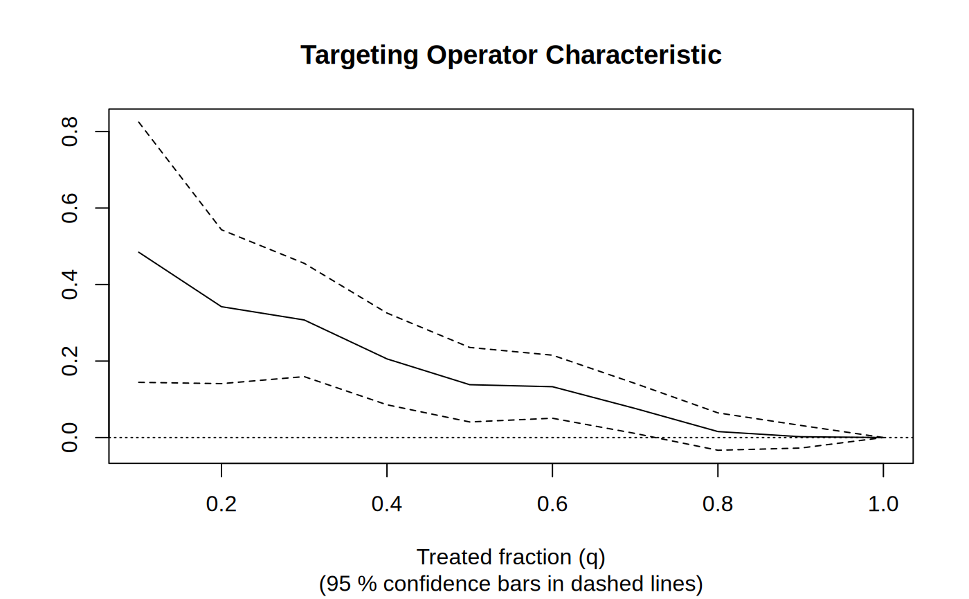
Figures reproduced from grf — Athey, Tibshirani & Wager — unofficial community showcase; all credit to the original authors.
The GRF 'introduction' vignette, distilled to a teaching recipe. Shows the shared API across forest types and where OOB predictions and variable importance come from. Unofficial summary.
Discuss the workflow (2)
Log in to join the discussion.
Perfect first-contact recipe. Showing the identical call shape across regression/quantile/causal forests is the fastest way to 'get' the package.
Would hand this to any new grad student. Clean.