
An observational ATE you can defend (balance → estimate → sensitivity)
Follow the analysis.
Select a node to explore the method
Treatment, covariates, outcome
Data preparation — shapes the raw inputs into what the estimator expects.
Assemble the design matrix; keep the outcome sealed until matching is done.
data("lalonde", package = "MatchIt")

Before using this step, make its assumptions and its output explicit. A useful peer note explains what you would check, what could go wrong, or what would change your interpretation.
Questions to explore- Which assumption matters most here, and what evidence could challenge it?
- What would you check before passing this output to the next step?
Choose a question to start your comment.
Peer discussion
- Bring your experience, a question, or a different perspective.
Log in to comment on this step.
matchit() — nearest-neighbour matching
Data preparation — shapes the raw inputs into what the estimator expects.
Match on the propensity score — the outcome-blind design stage.
m <- matchit(treat ~ age + educ + race + re74 + re75, lalonde, method="nearest")
Before using this step, make its assumptions and its output explicit. A useful peer note explains what you would check, what could go wrong, or what would change your interpretation.
Questions to explore- Which assumption matters most here, and what evidence could challenge it?
- What would you check before passing this output to the next step?
Choose a question to start your comment.
Peer discussion
- Bring your experience, a question, or a different perspective.
Log in to comment on this step.
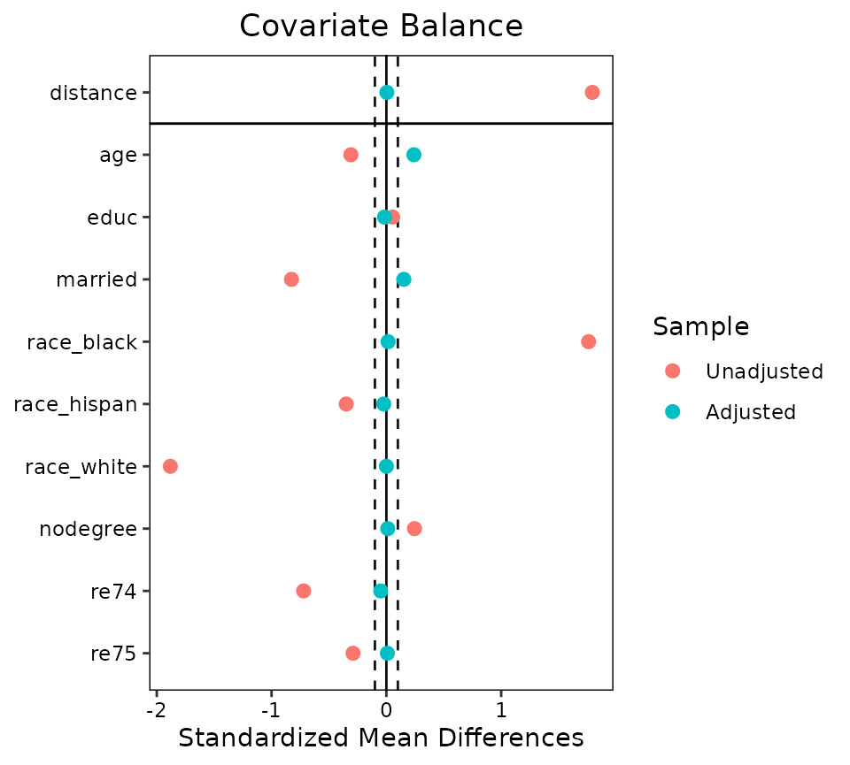
bal.tab() / love.plot() — cobalt
A pre-flight check — run this before trusting any estimate downstream.
Prove the matching worked: SMDs adjusted vs unadjusted, plus the Love plot.
bal.tab(m, un = TRUE); love.plot(m, thresholds = c(m = .1))
Before using this step, make its assumptions and its output explicit. A useful peer note explains what you would check, what could go wrong, or what would change your interpretation.
Questions to explore- Which assumption matters most here, and what evidence could challenge it?
- What would you check before passing this output to the next step?
Choose a question to start your comment.
Peer discussion
- Bring your experience, a question, or a different perspective.
Log in to comment on this step.
Estimate the ATT on matched data
The core estimate — where the causal quantity itself is computed.
Outcome model on match.data() with cluster-robust SEs.
fit <- lm(re78 ~ treat, data = match.data(m), weights = weights)
Before using this step, make its assumptions and its output explicit. A useful peer note explains what you would check, what could go wrong, or what would change your interpretation.
Questions to explore- Which assumption matters most here, and what evidence could challenge it?
- What would you check before passing this output to the next step?
Choose a question to start your comment.
Peer discussion
- Bring your experience, a question, or a different perspective.
Log in to comment on this step.
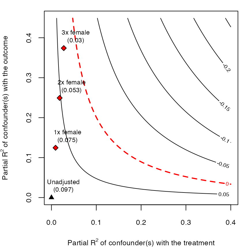
sensemakr() — robustness value + contours
Reporting — turn the numbers into a figure or table a reader can act on.
Report the robustness value + contour plots — how wrong could unconfoundedness be?
s <- sensemakr(fit, treatment="treat", benchmark_covariates="re74", kd=1:3)
plot(s)
Before using this step, make its assumptions and its output explicit. A useful peer note explains what you would check, what could go wrong, or what would change your interpretation.
Questions to explore- Which assumption matters most here, and what evidence could challenge it?
- What would you check before passing this output to the next step?
Choose a question to start your comment.
Peer discussion
- Bring your experience, a question, or a different perspective.
Log in to comment on this step.
Inputs & data
A binary treatment, the covariates to adjust for, and an outcome (e.g. the Lalonde job-training data).
Show data format & exampleHide example
Format — one row per unit: treatment W ∈ {0,1}, covariates X, outcome Y.
  W  age educ   race   re74  re78
  1   37   11  black     0  9930
  0   30   12  white  4100  4400
Figures reproduced from the package's official documentation — unofficial community showcase; all credit to the original authors.
Personal recipe — figures are from each package's public docs; this is my own composition, not affiliated with the package authors.
Selection-on-observables is an assumption, not a fact. This is the pipeline I actually run so the estimate survives review: design first (matching, outcome-blind), show balance, estimate, then state how strong an unobserved confounder would have to be to overturn it.
Discuss the workflow (0)
Log in to join the discussion.