

Two-stage least squares for instrumental-variables regression, with the modern LATE interpretation and rich diagnostics.
Input · what goes in
An outcome, one or more endogenous regressors, exogenous covariates, and instrument(s).
Show data format & exampleHide example
| y | educ (endog) | nearcollege (instr) |
|---|---|---|
| 6.1 | 12 | 0 |
| 6.9 | 16 | 1 |
| 5.8 | 11 | 0 |
| 7.2 | 14 | 1 |
Pipeline · the recipe
↑ Click any step in the diagram to read its logic, code, assumptions & discussion.
Load data and specify the IV formula
Data preparation — shapes the raw inputs into what the estimator expects.
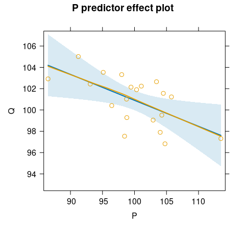
Use the classic Kmenta market data and write the two-part formula y ~ regressors | instruments separating endogenous and exogenous terms.
# Install:  install.packages("ivreg")
library("ivreg")
data("Kmenta", package = "ivreg")
# Q ~ P + D, with P endogenous; instruments are D, F, A
f <- Q ~ P + D | D + F + A
- No comments on this step yet — be the first.
Log in to comment on this step.
Fit the 2SLS / IV model
The core estimate — where the causal quantity itself is computed.
ivreg() estimates the structural equation by two-stage least squares using the supplied instruments.
fit <- ivreg(f, data = Kmenta)
- No comments on this step yet — be the first.
Log in to comment on this step.
Summary with diagnostic tests
Uncertainty quantification — standard errors, intervals, and aggregation.
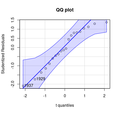
diagnostics=TRUE appends the three key tests: weak-instruments (large F means relevant instruments), Wu-Hausman (small p means OLS is biased, prefer IV), and Sargan (large p means the over-identifying instruments pass).
summary(fit, diagnostics = TRUE)
- No comments on this step yet — be the first.
Log in to comment on this step.
Output · what you get 2 figures
Figures reproduced from the package's official documentation — unofficial community showcase; all credit to the original authors.
Result · the numbers
⚠️ Unofficial community showcase of ivreg (docs). Not affiliated with the authors — all credit to Guido Imbens & coauthors; this summarizes public documentation.
What it does. Estimates causal effects when treatment is endogenous, using an instrument that affects treatment but not the outcome directly. ivreg fits the model by two-stage least squares (2SLS) with a clean outcome ~ covariates | instruments formula and diagnostics (weak instruments, Wu-Hausman, Sargan). How it works. The first stage projects the endogenous regressor onto the instrument; the second stage regresses the outcome on these fitted values. Assumptions. Instrument relevance, exclusion, independence, and—for the causal interpretation—monotonicity (no defiers). Imbens's contribution. Imbens & Angrist (1994, Econometrica) showed that, under monotonicity, IV/2SLS identifies the Local Average Treatment Effect—the effect for compliers whose treatment responds to the instrument—reframing what 2SLS actually estimates with heterogeneous effects.
What you get — 2SLS coefficient (the LATE for compliers) with standard errors and IV diagnostic tests.
Example output
Call:
ivreg(formula = Q ~ P + D | D + F + A, data = Kmenta)

Coefficients:
            Estimate Std. Error t value Pr(>|t|)
(Intercept) 94.63330    7.92084  11.947 1.08e-09 ***
P           -0.24356    0.09648  -2.524   0.0218 *
D            0.31399    0.04694   6.689 3.81e-06 ***

Diagnostic tests:
                 df1 df2 statistic  p-value
Weak instruments   2  16    88.025 2.32e-09 ***
Wu-Hausman         1  16    11.422  0.00382 **
Sargan             1  NA     2.983  0.08414 .
---
Residual standard error: 1.966 on 17 degrees of freedom
Multiple R-Squared: 0.7548, Adjusted R-squared: 0.726
Discussion (0)
Log in to join the discussion.