

Preprocesses observational data by matching treated and control units on covariates, so downstream models depend less on modeling assumptions.
Input · what goes in
A data frame with a binary treatment indicator and the covariates to balance on.
Show data format & exampleHide example
| treat | age | educ | married |
|---|---|---|---|
| 1 | 37 | 11 | 1 |
| 0 | 22 | 9 | 0 |
| 1 | 30 | 12 | 1 |
| 0 | 45 | 14 | 0 |
Pipeline · the recipe
↑ Click any step in the diagram to read its logic, code, assumptions & discussion.
Load MatchIt and the lalonde data
Data preparation — shapes the raw inputs into what the estimator expects.
Bring in the package and the canonical Lalonde job-training observational dataset.
# Install:  install.packages("MatchIt")
library("MatchIt")
data("lalonde")
head(lalonde)
- No comments on this step yet — be the first.
Log in to comment on this step.
Run 1:1 nearest-neighbor PS matching
The core estimate — where the causal quantity itself is computed.
Fit a logistic propensity score and match each treated unit to its nearest control without replacement.
m.out1 <- matchit(treat ~ age + educ + race + married +
                    nodegree + re74 + re75,
                  data = lalonde,
                  method = "nearest",
                  distance = "glm")
- No comments on this step yet — be the first.
Log in to comment on this step.
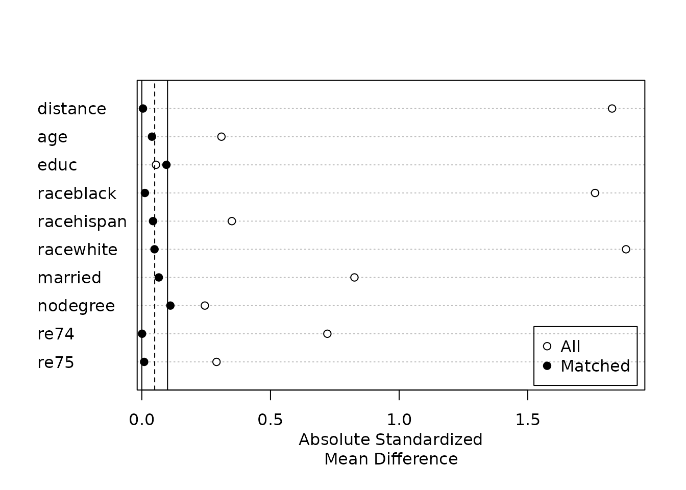
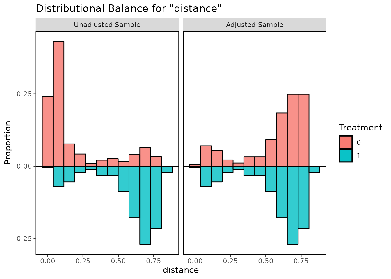
Assess covariate balance
A pre-flight check — run this before trusting any estimate downstream.
Inspect standardized mean differences before and after matching to check that matching reduced imbalance.
summary(m.out1)
plot(m.out1, type = "density", interactive = FALSE)
- No comments on this step yet — be the first.
Log in to comment on this step.
Extract the matched dataset
Data preparation — shapes the raw inputs into what the estimator expects.
Pull out the matched sample with matching weights and subclass identifiers for the outcome model.
m.data <- match.data(m.out1)
- No comments on this step yet — be the first.
Log in to comment on this step.
Estimate the ATT
The core estimate — where the causal quantity itself is computed.
Fit a weighted outcome regression and use marginaleffects to get the average treatment effect on the treated with cluster-robust SEs.
library("marginaleffects")
fit <- lm(re78 ~ treat * (age + educ + race + married +
                           nodegree + re74 + re75),
          data = m.data, weights = weights)
avg_comparisons(fit, variables = "treat",
                vcov = ~subclass,
                newdata = subset(m.data, treat == 1))
- No comments on this step yet — be the first.
Log in to comment on this step.
Output · what you get 4 figures


Figures reproduced from the package's official documentation — unofficial community showcase; all credit to the original authors.
Result · the numbers
⚠️ Unofficial community showcase of MatchIt (docs). Not affiliated with the authors — all credit to Gary King & coauthors; this summarizes public documentation.
What it does: MatchIt selects matched subsamples of treated and control units with similar covariate distributions, so that a subsequent parametric model (e.g. a regression) is less sensitive to specification. How it works: It supports many methods—nearest-neighbor and optimal propensity-score matching, exact and coarsened exact matching, genetic matching, and full/subclassification—then reports covariate balance (standardized mean differences, eCDF, Love plots) before and after. Effects are estimated on the matched data, typically with weights and robust/cluster-robust standard errors. Assumptions: Causal interpretation requires unconfoundedness (selection on observables) and overlap/common support between groups; matching only addresses observed covariates, not unmeasured confounding. It implements Ho, Imai, King & Stuart's 'matching as nonparametric preprocessing' recommendations.
What you get — A matched dataset (with weights/subclasses) plus balance diagnostics for estimating treatment effects.
Example output
Call:
matchit(formula = treat ~ age + educ + race + married + nodegree +
    re74 + re75, data = lalonde, method = "nearest", distance = "glm")

Summary of Balance for All Data:
           Means Treated Means Control Std. Mean Diff. Var. Ratio eCDF Mean eCDF Max
distance          0.5774        0.1822          1.7941     0.9211    0.3774   0.6444
age              25.8162       28.0303         -0.3094     0.4400    0.0813   0.1577
educ             10.3459       10.2354          0.0550     0.4959    0.0347   0.1114
raceblack         0.8432        0.2028          1.7615          .    0.6404   0.6404
married           0.1892        0.5128         -0.8263          .    0.3236   0.3236
re74           2095.5737     5619.2365         -0.7211     0.5181    0.2248   0.4470

Summary of Balance for Matched Data:
           Means Treated Means Control Std. Mean Diff. Var. Ratio eCDF Mean eCDF Max
distance          0.5774        0.3629          0.9739     0.7566    0.1321   0.4216
age              25.8162       25.3027          0.0718     0.4568    0.0847   0.2541
married           0.1892        0.2108         -0.0552          .    0.0216   0.0216
re74           2095.5737     2342.1076         -0.0505     1.3289    0.0469   0.2757

Sample Sizes:
          Control Treated
All           429     185
Matched       185     185
Unmatched     244       0
Discussion (2)
Log in to join the discussion.
Matching as the design stage — outcome-free — is the discipline people skip. MatchIt makes it the path of least resistance.
And match.data() → any outcome model. Pairs perfectly with cobalt for the balance plots.
Nearest, optimal, full, genetic — all behind one matchit() call. Great teaching tool.