

Build a weighted 'synthetic' control from untreated units to estimate the effect of a single treated case over time.
Input · what goes in
Panel data: unit IDs, time periods, an outcome, and predictor variables; one treated unit and a donor pool.
Show data format & exampleHide example
| unit | year | gdp | invest |
|---|---|---|---|
| 1 | 1990 | 100 | 22 |
| 1 | 1991 | 104 | 23 |
| 2 | 1990 | 88 | 19 |
| 2 | 1991 | 90 | 20 |
Pipeline · the recipe
↑ Click any step in the diagram to read its logic, code, assumptions & discussion.
Prepare the panel with dataprep()
Data preparation — shapes the raw inputs into what the estimator expects.
Package the Basque panel into the X0/X1/Z0/Z1 matrices: Basque Country (region 17) is treated, the other 16 regions form the donor pool.
# Install:  install.packages("Synth")
library(Synth)
data(basque)
dp <- dataprep(
  foo = basque,
  predictors = c("school.illit","school.prim","school.med",
                 "school.high","school.post.high","invest"),
  predictors.op = "mean",
  dependent = "gdpcap",
  unit.variable = "regionno",
  time.variable = "year",
  treatment.identifier = 17,
  controls.identifier = c(2:16,18),
  time.predictors.prior = 1964:1969,
  time.optimize.ssr = 1960:1969,
  unit.names.variable = "regionname",
  time.plot = 1955:1997)
- No comments on this step yet — be the first.
Log in to comment on this step.
Optimize the donor weights
The core estimate — where the causal quantity itself is computed.
synth() solves the nested optimization for the unit weights W and predictor weights V that minimize pre-treatment outcome distance.
so <- synth(data.prep.obj = dp)
- No comments on this step yet — be the first.
Log in to comment on this step.
Donor weights and predictor balance tables
Reporting — turn the numbers into a figure or table a reader can act on.
synth.tab() returns tab.w (donor weights) and tab.pred (treated vs synthetic predictor means).
tabs <- synth.tab(dataprep.res = dp, synth.res = so)
tabs$tab.w     # donor weights
tabs$tab.pred  # predictor balance
- No comments on this step yet — be the first.
Log in to comment on this step.
Path and gaps plots
Reporting — turn the numbers into a figure or table a reader can act on.
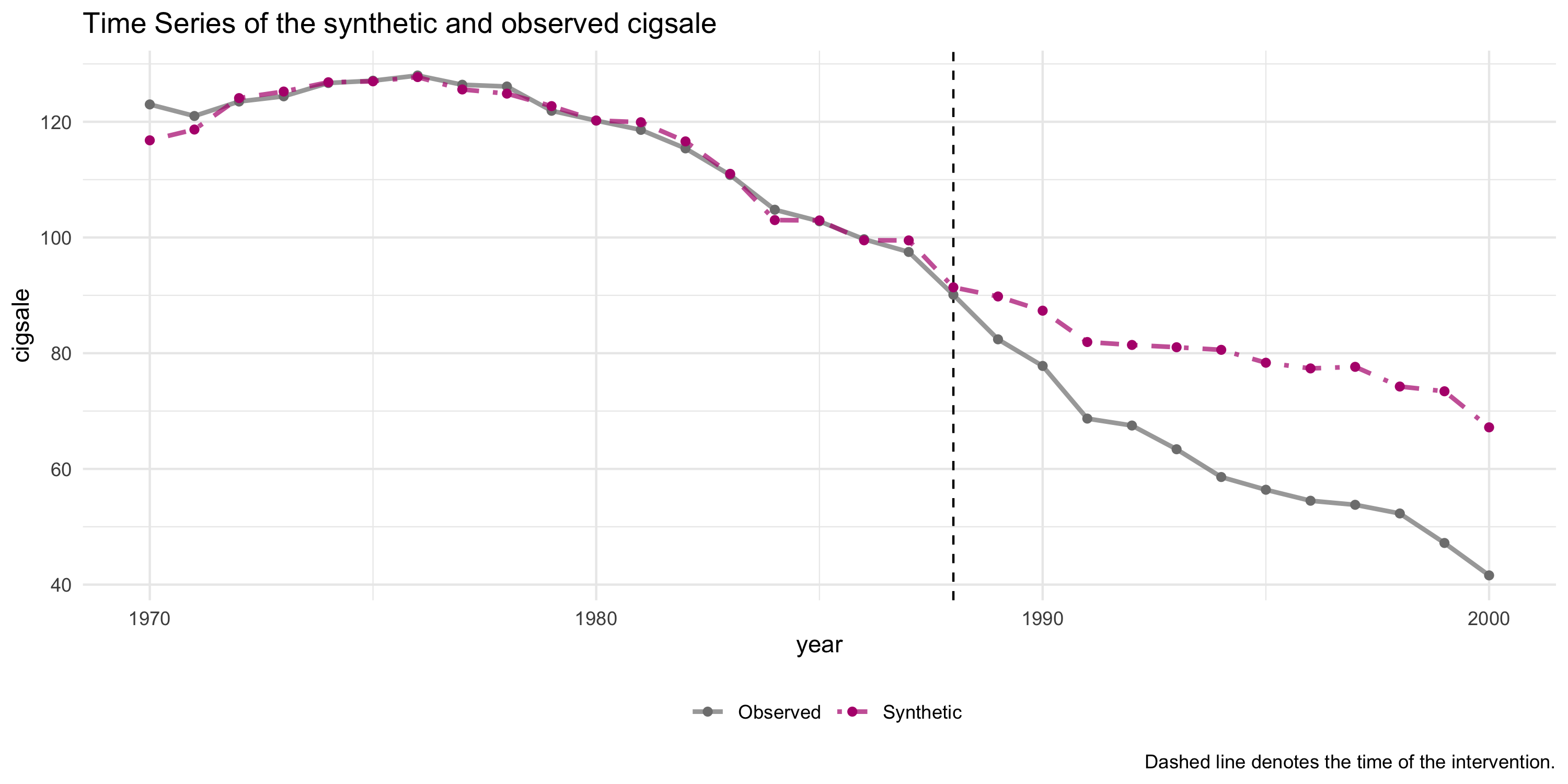
Visualize treated vs synthetic GDP over time and the estimated treatment gap after 1970.
path.plot(synth.res = so, dataprep.res = dp,
Ylab = "real per-capita GDP", Xlab = "year")
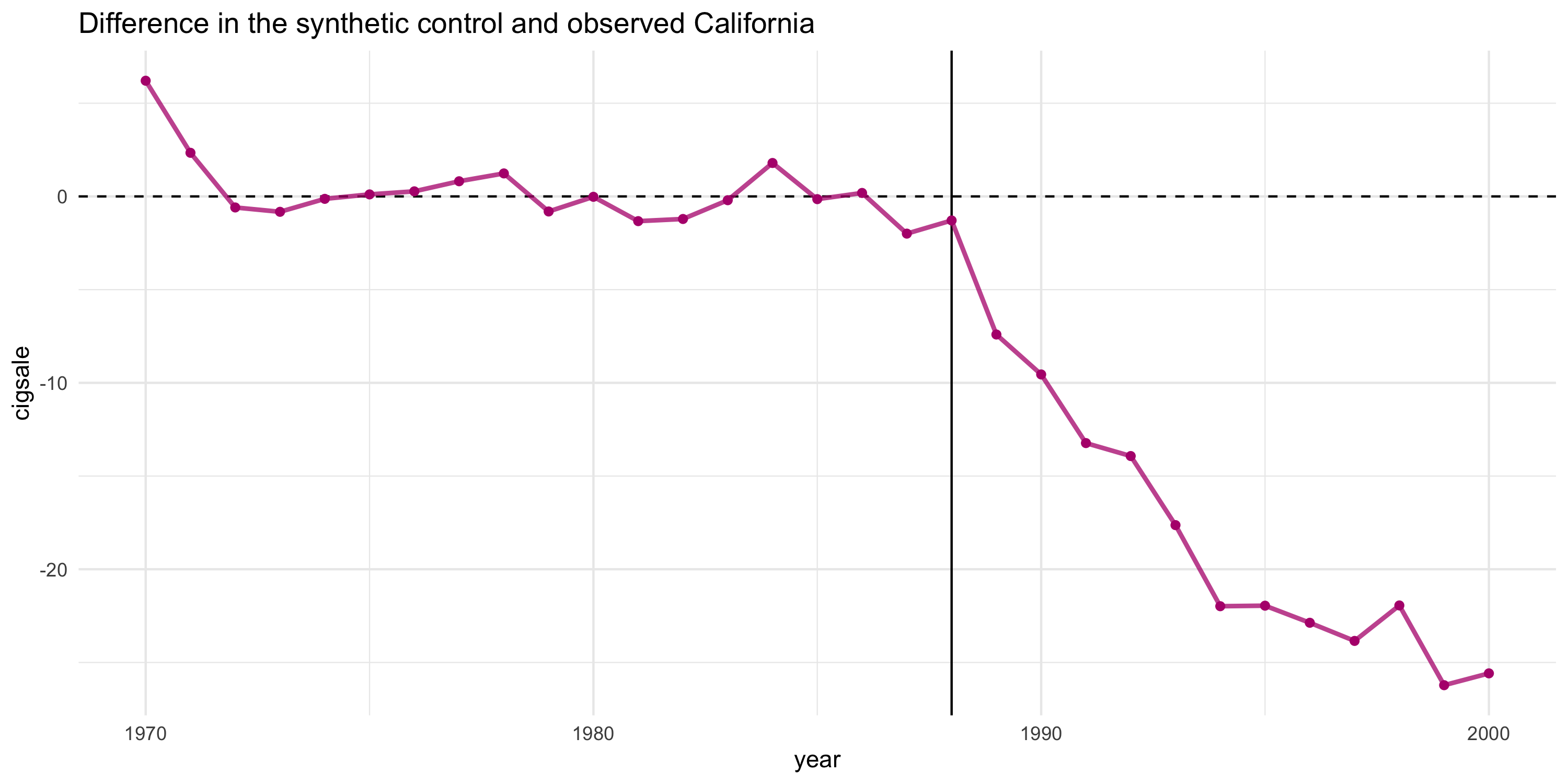
gaps.plot(synth.res = so, dataprep.res = dp,
Ylab = "gap in per-capita GDP", Xlab = "year")
- No comments on this step yet — be the first.
Log in to comment on this step.
Output · what you get 2 figures
Figures reproduced from the package's official documentation — unofficial community showcase; all credit to the original authors.
Result · the numbers
⚠️ Unofficial community showcase of Synth (docs). Not affiliated with the authors — all credit to Guido Imbens & coauthors; this summarizes public documentation.
What it does. When one unit (a state, country, firm) is treated, Synth constructs a counterfactual by optimally weighting comparison units so the synthetic unit matches the treated unit's pre-treatment outcomes and predictors; the post-treatment gap is the estimated effect. How it works. It solves a nested optimization for non-negative weights that sum to one, minimizing pre-period discrepancy, then projects the synthetic control forward. Assumptions. No interference/spillovers to controls, no anticipation, and a convex combination of donors that tracks the treated unit pre-treatment. Imbens's contribution. The Synth package implements Abadie, Diamond & Hainmueller (2010); Imbens is a leading figure in this design-based panel literature and co-developed Synthetic Difference-in-Differences (Arkhangelsky, Athey, Hirshberg, Imbens & Wager, 2021), which unifies synthetic control with difference-in-differences.
What you get — Donor weights and a treated-vs-synthetic outcome gap (the estimated treatment effect path).
Example output
$tab.pred
                          Treated Synthetic Sample Mean
school.illit               39.888   256.337     170.786
school.prim              1031.742  2730.104    1127.186
school.med                 90.359   223.340      76.260
school.high                25.728    63.437      24.235
invest                     24.647    21.583      21.424

$tab.w
        w.weights unit.names unit.numbers
2           0.000  Andalucia            2
10          0.851  Cataluna            10
14          0.149     Madrid           14
Discussion (0)
Log in to join the discussion.